introduction
estrannaise.js uses several mathematical concepts under the hood. It combines pharmacokinetics compartments models with Markov Chain Monte Carlo (MCMC) to infer the pharmacokinetics parameters of estradiol using Bayesian generative models, both hierarchical and non-hierarchical, that account for the variability found in data both within and across studies. The following is the list of the ingredients and the recipe behind it.
pharmacokinetics models
The pharmacokinetics models used in estrannaise.js are traditional compartments models. For now we use only linear first-order ordinary differential equations (ODEs). These models are used to describe the absorption, distribution, metabolism, and excretion of drugs in the body.
simple 3-compartments model
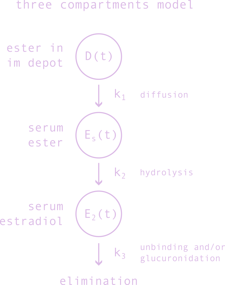
To begin, we model the metabolism of an intramuscular depot of estradiol ester by a very simple 3-compartments model which includes three processes. The first compartment, shown on the right, models the content of estradiol ester in the depot, the second the serum concentration of the estradiol ester, and the third the serum concentration of estradiol. The first process is the diffusion of the ester out of the oil and into systemic circulation, the second process is the hydrolysis of the ester into estradiol by esterases in the liver, and the third process is the elimination of estradiol by the body, mainly by glucuronidation and conjugation followed by excretion by the kidneys, and to a lesser extent by the liver and the intestines. For a portion of the estradiol this last process must be preceeded by the unbinding of the estradiol from the estrogen receptor which happens on a different time-scale.
The differential equation for this model in the presence of multiples
doses \(d_i\) at times \(t_i\) is given by
\begin{equation}\label{eq:3C}\begin{split}
\frac{dD(t)}{dt} &= -k_1 D(t) + \sum_i d_i \delta(t - t_i),\\
\frac{dE_s(t)}{dt} &= k_1 D(t) - k_2 E_s(t),\\
\frac{dE_2(t)}{dt} & = k_2 E_s(t) - k_3 E_2(t),\\
D(0) &= E_s(0) = E_2(0) = 0,
\end{split}\end{equation}
where \(\delta(t)\) is the Dirac delta function. We have assumed without
loss of generality that all \(t_i > 0\)'s. One can consider a single dose \(d\)
at a time that approaches zero in order to mimick a situation with initial condition
\(D(0) = d\). The serum concentration of estradiol
\(E_2^{sd}(t)\) after the injection of a single dose \(d\) at time
\(t=0\) is given by (see appendix for details)
where the Heaviside function \begin{equation*} H(t) = \begin{cases} 0 & \text{if } t < 0,\\ 1 & \text{if } t \geq 0, \end{cases} \end{equation*} insures the solution is zero for \(t < 0\). This assumes there were no baseline serum level prior to the injection. For multiple doses we have the following multi-dose solution \begin{equation*}\begin{split} E_2^{md3C}&(t~\vert~\lbrace d_i, t_i\rbrace, k_1, k_2, k_3)=\sum_i E^{sd3C}_2(t - t_i~\vert~d_i, k_1, k_2, k_3),\\ &=k_1 k_2\sum_i d_i H(t - t_i)\left[\frac{e^{-k_1 (t - t_i)}}{(k_1 - k_2)(k_1 - k_3)} - \frac{e^{-k_2(t - t_i)}}{(k_1 - k_2)(k_2 - k_3)} + \frac{e^{-k_3(t - t_i)}}{(k_1 - k_3)(k_2 - k_3)}\right]. \end{split}\end{equation*} This solution is nothing but the expression of the superposition principle of linear ODEs. By the same principle, we can just as well let the parameters \(k_1, k_2, k_3\) vary from dose to dose, in effect simulating the the use of a combination of different esters at different times. This multi-dose, multi-ester solution is given by \begin{equation*}\begin{split} E_2^{mde3C}&\left(t~\vert~\lbrace d_i, t_i, k_{1i}, k_{2i}, k_{3i}\rbrace\right)=\sum_i E^{sd3C}_2(t - t_i~\vert~d_i, k_{1i}, k_{2i}, k_{3i}),\\ &=\sum_i d_i k_{1i} k_{2i} H(t - t_i)\left[\frac{e^{-k_{1i} (t - t_i)}}{(k_{1i} - k_{2i})(k_{1i} - k_{3i})} - \frac{e^{-k_{2i}(t - t_i)}}{(k_{1i} - k_{2i})(k_{2i} - k_{3i})} + \frac{e^{-k_{3i}(t - t_i)}}{(k_{1i} - k_{3i})(k_{2i} - k_{3i})}\right]. \end{split}\end{equation*} Note that technically all esters should share the same elimination rate \(k_3\), but we can relax this assumption by keeping in mind that this model does not perfectly capture reality and process rates in a model that tries to collapse reality into 3 compartments will inevitably have to bleed into, and compensate for, each others' insufficiencies during curve-fitting.
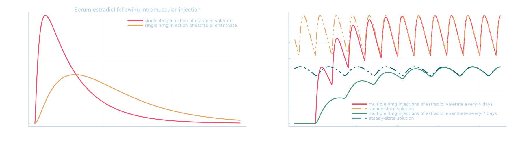
steady state solution under repeated doses
Following the repeated injection of the same dose at regular intervals, serum estradiol levels will settle into a periodic pattern called the steady-state solution. The steady-state solution \(E_2^{ss3C}(t)\) is given by the multi-dose solution with an infinite train of doses \(d\) at regular intervals \(T\) which we write \begin{equation}\label{eq:infinitesumsteadystate3C}\begin{split} E_2^{ss3C}(t) &= \sum_{i=-\infty}^{\infty} E^{sd3C}_2(t - iT~\vert~d, k_1, k_2, k_3),\\ &= d k_1 k_2\sum_{i=-\infty}^\infty H(t - iT)\left[\frac{e^{-k_1 (t - iT)}}{(k_1 - k_2)(k_1 - k_3)} - \frac{e^{-k_2(t - iT)}}{(k_1 - k_2)(k_2 - k_3)} + \frac{e^{-k_3(t - iT)}}{(k_1 - k_3)(k_2 - k_3)}\right]. \end{split}\end{equation} The dependence on \(i\) takes the form of the following infinite sum \begin{equation*} S = \sum_{i=-\infty}^\infty H(t - iT) e^{k T i}. \end{equation*} Note that for a given \(t\), the Heaviside function is non-zero only when \(t - iT \ge 0\) (remember we define \(H(0) = 1\)) and therefore when \(i \le \lfloor t/T \rfloor\) where \(\lfloor~.\rfloor\) is the floor function which rounds toward \(-\infty\). We can therefore truncate the infinite sum \begin{equation*} S = \sum_{i=-\infty}^{\lfloor t/T\rfloor}e^{k T i}. \end{equation*} Now shift the summation by introducing the change of variable \(i \rightarrow i + \lfloor t/T\rfloor\), \begin{equation*} S = e^{k T\lfloor t/T\rfloor} \sum_{i=-\infty}^0 e^{k T i}, \end{equation*} and flip the sum by sending \(i \rightarrow -i\) to get \begin{equation*} S = e^{k T\lfloor t/T\rfloor} \sum_{i=0}^\infty e^{-k T i}. \end{equation*} Since \(e^{-kT}\) is strictly smaller than 1 we use the geometric series which finally gives us \begin{equation}\label{eq:ssgeomidentity} S = \frac{e^{k T\lfloor t/T\rfloor}}{1 - e^{-kT}}. \end{equation} Using \eqref{eq:ssgeomidentity} for the three exponential terms in \eqref{eq:infinitesumsteadystate3C} we finally obtain an explicit expression for the steady-state solution
The steady-state solution gives us easy access to the exposure, also called the area under the curve (AUC). Since \(\int_0^T e^{-k t} = (1 - e^{-k T})/k\) the numerators in \eqref{eq:steadystate3C} cancel the steady state factor in the denominators and therefore the AUC over one period \begin{equation*}\begin{split} \text{AUC}_T = \int_0^T E_2^{ss3C}(t) dt &= d k_1 k_2\left(\frac{1}{k_1(k_1 - k_2)(k_1-k_3)} - \frac{1}{k_2(k_1-k_2)(k_2-k_3)} + \frac{1}{k_3(k_1-k_3)(k_2-k_3)}\right),\\ &= d k_1 k_2\frac{k_2 k_3 (k_2 - k_3) - k_1 k_3(k_1 - k_3) + k_1 k_2(k_1 - k_2)}{k_1 k_2 k_3(k_1 - k_2)(k_1-k_3)(k_2 - k_3)},\\ & = \frac{d}{k_3}. \end{split}\end{equation*} Note how it is independent of the rates \(k_1, k_2\). The average level at steady state is therefore \begin{equation*} \overline{E^{ss}_2} = \frac{\text{AUC}_T}{T} = \frac{d}{k_3 T}. \end{equation*} This highlights the fact that average levels only depend on the elimination rate of estradiol by the body and the dose per-\(T\) and are therefore independent of the specific ester used. Reality is more messy than this simple model and this messiness will be captured by the fact that the rate \(k_3\) we will infer later will be different for different esters. For the purpose of hormonotherapy we are often interested in levels "at trough", namely at their lowest just before the next injection. This is given by the value of serum estradiol at the beginning of each period in the steady state, for example at \(t = 0\), and thus \begin{equation*} E^{tr}_2 = E^{ss}_2(0) = d k_1 k_2\left[\frac{1}{(1 - e^{-k_1T})(k_1 - k_2)(k_1 - k_3)} - \frac{1}{(1 - e^{-k_2T})(k_1 - k_2)(k_2 - k_3)} + \frac{1}{(1 - e^{-k_3T})(k_1 - k_3)(k_2 - k_3)}\right]. \end{equation*} One interesting point to note is that this is not the "true" trough, but a very close approximation. The "true" trough is reached a little after the injection. We do not show this but the derivative is indeed always negative or zero at \(t = 0\). One can check that at first order in \(k_1, k_2, k_3\) with \(T\) of order 1 the derivative is approximately \(-d k_1 k_2 T/12\) which is negative for non-zero rates. Intuitively this is due to the fact that there is a delay introduced by rates of diffusion and cleavage of the ester and therefore the rate of increase of serum estradiol caused by the new depot does not immediately compensate for the rate of elimination. There is inertia in the system.
3-compartments model for patches
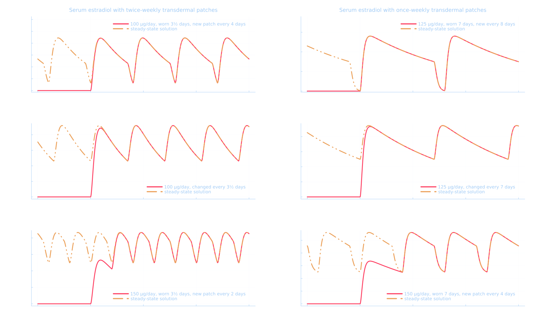
We can use the 3-compartment model to model the pharmacokinetic of transdermal estradiol. Patches are made of a backing layer, a reservoir of estradiol, and a membrane that controls the rate of diffusion of estradiol into the skin. \(D(t)\) can now stand for the amount of estradiol in the patch, the rate \(k_1\) for the rate of diffusion across the membrane, \(E_s(t)\) for the amount of estradiol in the skin, and \(k_2\) the combined rate of diffusion and absorption of estradiol across the skin and into capillaries. The differential equation is thus given \eqref{eq:3C} once again. One particularity of using patches is that one usually replaces it once or twice a week. Denote the length of time the patch is worn \(W\). When \(t = W\) is reached the patch is removed and \(D(W)\) is set to zero. From this point on \(E_s(t)\) and \(E_2(t)\) act as a 2-compartments model with initial conditions \(E_s(W)\) and \(E_2(W)\). To get \(E_2(t)\) for \(t \ge W\) can use \eqref{eq:thirdcompartmentsolution} with where all \(d_i=0\), and \(d_0^s = E_s(W)\) and \(d_0^2 = E_2(W)\) both at \(t_0 = W\). We can immediately write
steady state solution for patches
The pieceweise form of the single patch solution \eqref{eq:patch3C} introduces one small complication when we want to compute the steady state solution. Intuitively, the steady-state at a time \(t\) is given by the sum of all contributions from the solution after \(t \ge W\) plus the contribution of the currently worn patch. Let's rewrite \eqref{eq:patch3C} in a more convenient form reminescent of the multi-dose solution \begin{equation*}\begin{split} E^{ssp3C}_2(t) &= \sum_{i=-\infty}^{\infty} E^{p3C}_2(t - iT),\\ &= \sum_{i=-\infty}^{\infty} E_2^{sd3C}(t - iT) H(t - iT) H^+(W - t + iT) \\ & + \sum_{i=-\infty}^{\infty}\frac{k_2 E_s^{sd3C}(W)}{k_2 - k_3}H(t - W - i T)\left[e^{-k_3(t - W -iT)} - e^{-k_2(t - W - iT)}\right] + E_2^{sd3C}(W) H(t - W - i T) e^{-k_3 (t - W - iT)}, \end{split}\end{equation*} where \(H^+(x) = 1 - H(-x)\), meaning that contrary to \(H(0) = 1\) this version of the Heaviside function is defined such that \(H^+(0) = 0\) We need it to respect the strict inequality \(t < W\) in the first part of \eqref{eq:patch3C}. The identity \eqref{eq:ssgeomidentity} gives us the second infinite sum, so let's focus on the first. The product of Heaviside functions \(H(t - iT) H^+(W - t + iT)\) is non-zero only when $$t - iT \ge 0 \text{ and } W - t + iT > 0,$$ which implies $$ \lfloor(t - W)/T\rfloor < i \le \lfloor t/T\rfloor.$$ The dependence on \(i\) in this second infinite sum takes the form \begin{equation*}\begin{split} R &= \sum_{i=-\infty}^\infty e^{k T i} H(t - iT) H^+(W - t + iT),\\ &=\sum_{i=\lfloor(t - W)/T\rfloor + 1}^{\lfloor t/T\rfloor} \left(e^{k T}\right)^i,\\ &=\frac{e^{k T\lfloor t/T\rfloor} - e^{k T\lfloor(t - W)/T\rfloor}}{1 - e^{-k T}}, \end{split}\end{equation*} and therefore the steady-state solution for patches
This solution is once again periodic with period \(T\). Figure X shows the convergence of a solution that is the sum of single patch solutions to the exact curve given by the steady-state patch solution. Note that in the bottom two plots \(T < W\) which represents an unrealistic situation where new patches are added faster than old patches are removed and would lead to an infinite accumulation of patches on one's body. They only serves to illustrate the validity of the steady-state solution in all cases.
inference with simple gaussian model
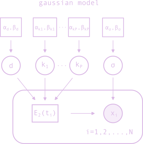
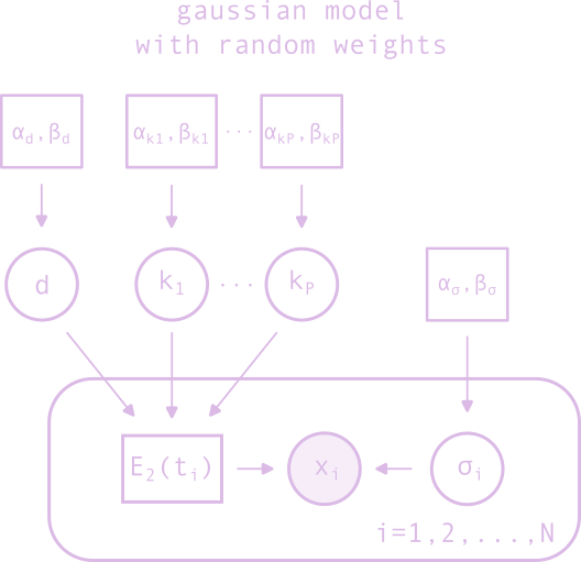
Given a data set consisting of a series of measurements of serum estradiol levels following the injection of a single dose, we can write down a simple generative model for the data where each measurement is assumed to be independent and normally distributed around the deterministic value given by the single-dose solution of the 3-compartments model. The four parameters of the pharmacokinetic model are the dose \(d\), and the three rate constants \(k_1, k_2, k_3\). We assume that each of them is distributed according to a gamma distribution. There is a fifth parameter, the standard deviation of the normal distribution, which we assume is distributed according to an inverse gamma distribution. The generative model is therefore given by \begin{equation*}\begin{split} d &\sim \operatorname{Gamma}(\alpha_d, \beta_d),\\ k_1 &\sim \operatorname{Gamma}(\alpha_{k_1}, \beta_{k_1}),\\ k_2 &\sim \operatorname{Gamma}(\alpha_{k_2}, \beta_{k_2}),\\ k_3 &\sim \operatorname{Gamma}(\alpha_{k_3}, \beta_{k_3}),\\ \sigma &\sim \operatorname{InvGamma}(\alpha_{\sigma}, \beta_{\sigma}),\\ x_i &\sim \operatorname{Normal}\left(E_2^{sd3C}(t_i~\vert~d, k_1, k_2, k_3), \sigma\right),\quad i=1,\ldots,N. \end{split}\end{equation*} The plate model is shown in Figure 2. If the standard deviation \(\sigma_i\) is available then we can simply use those explicitly instead of specifying a prior on a unique \(\sigma\). The hyperparameters \(\alpha\)'s and \(\beta\)'s that control the rates can be use to enforce prior knowledge about them. For example, if we know that the half-life of estradiol is just short of 24 hours, we can set \(\alpha_{k_3} = \beta_{k_3} = 1\) which would give us a mean of 24 hours for the half-life of estradiol. Indeed the mean of a gamma distribution is given by \(\alpha/\beta\). Since we know that esterase rapidly cleave the ester into estradiol in a matter of hours we can set \(1 < \beta_{k_2} < 10 \) with \(\alpha_{k_2}=1\). The rate of diffusion of the ester out of the depot varies, but we can make a rough guess that the time-scale is on the order of a few days up to a few months, and we can therefore set \(\alpha_{k_1}=1\) and \(\beta_{k_1}=1/5\). To set the hyperparameters of the inverse gamma prior over the standard deviation we eyeball the data, notice that there is a large range of variation, and set it so that its mean is somewhere between 10 and 100. Since the mean of an inverse gamma distribution is given by \(\beta/(\alpha - 1)\) we can set \(\alpha_{\sigma}=2\) and \(\beta_{\sigma}=20\). One reason to choose the inverse gamma distribution over the gamma distribution is that it has a long tail but also suppresses small values, which helps prevent the collapse of the posterior distribution to small values of \(\sigma\).
Another possibilities for a prior on the standard deviation is to use a non-informative prior like the Jeffreys prior of the reference prior. Both the Jeffreys and reference priors are given by \begin{equation*} P(\sigma) \propto \frac{1}{\sigma}. \end{equation*} Unfortunately, the this is an improper proper distribution (it integral diverges). While the resulting posterior is proper it can cause problems with automatic MCMC samplers like the ones we use as part of Julia's Turing.jl package. We will therefore approximate this prior by a proper prior which gives something close to a \(1/\sigma\) behavior for and medium \(\sigma\) and a long exponential tail for large \(\sigma\). The gamma distribution with a small value of for both \(\alpha\) and \(\beta\) is a good candidate for this and we can set for example \(\alpha_{\sigma} = 1/10\) and \(\beta_{\sigma} = 1/100\).
The explicit formula for the generative model is \begin{equation*}\begin{split} & P(\lbrace x_i\rbrace, d, k_1, k_2, k_3, \sigma~\vert~\alpha, \beta) = P(d)P(k_1)P(k_2)P(k_3)P(\sigma)\prod_{i=1}^N P(x_i~\vert~d, k_1, k_2, k_3, \sigma),\\ &= \frac{\beta_d^{\alpha_d}}{\Gamma(\alpha_d)}d^{\alpha_d - 1}e^{-\beta_d d}\frac{\beta_{k_1}^{\alpha_{k_1}}}{\Gamma(\alpha_{k_1})}k_1^{\alpha_{k_1} - 1}e^{-\beta_{k_1} k_1}\frac{\beta_{k_2}^{\alpha_{k_2}}}{\Gamma(\alpha_{k_2})}k_2^{\alpha_{k_2} - 1}e^{-\beta_{k_2} k_2}\frac{\beta_{k_3}^{\alpha_{k_3}}}{\Gamma(\alpha_{k_3})}k_3^{\alpha_{k_3} - 1}e^{-\beta_{k_3} k_3} \\ &\times\frac{\beta_{\sigma}^{\alpha_{\sigma}}}{\Gamma(\alpha_{\sigma})}\sigma^{-\alpha_{\sigma} - 1}e^{-\beta_{\sigma}/\sigma}\prod_{i=1}^N \frac{1}{\sqrt{2\pi\sigma^2}}e^{-\frac{1}{2\sigma^2}\left(x_i - E_2^{sd3C}(t_i~\vert~d, k_1, k_2, k_3)\right)^2}. \end{split}\end{equation*} The posterior distribution over the parameters of the model is given by \begin{equation*}\begin{split} P(d, k_1, k_2, k_3, \sigma~\vert~\lbrace x_i\rbrace, \alpha, \beta) &= \frac{P(\lbrace x_i\rbrace, d, k_1, k_2, k_3, \sigma~\vert~\alpha, \beta)}{P(\lbrace x_i\rbrace~\vert~\alpha, \beta)},\\ &= \frac{P(\lbrace x_i\rbrace~\vert~d, k_1, k_2, k_3, \sigma) P(d, k_1, k_2, k_3, \sigma~\vert~\alpha, \beta)}{\int P(\lbrace x_i\rbrace~\vert~d, k_1, k_2, k_3, \sigma) P(d, k_1, k_2, k_3, \sigma~\vert~\alpha, \beta)~d\sigma~dk_3~dk_2~dk_1~dd}. \end{split}\end{equation*}
interlude
\(D_3\) symmetry of the \(E_2\) curve
Here's a fun fact about the the single-dose solution \(E^{sdEC}_2\) and the multi-dose solution \(E^{mdEC}_2\) with all \(d_i\) equal. Let's use \(E_2\) to denote either of them and omit the time variable for brevity. The function \(E_2\) is invariant under 5 different transformations of its parameters, or 6 if we include the trivial one, called the identity and denoted by \(\operatorname{id}\). Notice first that interchanging \( k_1 \leftrightarrow k_2\) leaves the solution unchanged since the first and second terms transform into each other. Let's call this transformation \(\operatorname{T}_1\), \begin{equation*}\begin{split} \operatorname{T}_1\left[E_2(d, k_1, k_2, k_3)\right] &= E_2(d, k_2, k_1, k_3),\\ &= E_2(d, k_1, k_2, k_3). \end{split}\end{equation*} The second transformation is the interchange of \(k_1 \leftrightarrow k_3\), which we call \(\operatorname{T}_2\). By itself it doesn't leave \(E_2\) invariant unless we simultaneously substitute \(d\rightarrow dk_1/k_3\). Indeed, with a tiny bit of algebra we find \begin{equation*}\begin{split} \operatorname{T}_2\left[E_2\right] &= E_2\left(d k_1/k_3, k_3, k_2, k_1\right),\\ &= E_2(d, k_1, k_2, k_3). \end{split}\end{equation*} With \(\operatorname{T}_1\) and \(\operatorname{T}_2\) in our possession we can generate the remaining transformations. For example, applying \(\operatorname{T}_2\) followed by \(\operatorname{T}_1\) or vis-versa gives us the transformation \(\operatorname{T}_3\) and \(\operatorname{T}_4\). Omitting the brackets for brevity, \begin{equation*}\begin{split} \operatorname{T}_3 E_2 = \operatorname{T}_1\operatorname{T}_2E_2 &= E_2(dk_1/k_3, k_2, k_3, k_1),\\ & = E_2(d, k_1, k_2, k_3), \end{split}\end{equation*} and \begin{equation*}\begin{split} \operatorname{T}_4 E_2 = \operatorname{T}_2\operatorname{T}_1E_2 &= E_2(dk_2/k_3, k_3, k_1, k_2),\\ & = E_2(d, k_1, k_2, k_3). \end{split}\end{equation*} The final transformation implies applying \(\operatorname{T}_3\) followed by \(\operatorname{T}_2\) which incidentally is the same as applying \(\operatorname{T}_4\) followed by \(\operatorname{T}_1\). We call this transformation \(\operatorname{T}_5\), and we can verify with some more algebra that \begin{equation*}\begin{split} \operatorname{T}_5 E_2 &= \operatorname{T}_2\operatorname{T}_1\operatorname{T}_2E_2,\\ &= \operatorname{T}_1\operatorname{T}_2\operatorname{T}_1E_2,\\ &= E_2(dk_2/k_3, k_1, k_3, k_2),\\ &= E_2(d, k_1, k_2, k_3). \end{split}\end{equation*} It is easy to show that both \(\operatorname{T}_1\) and \(\operatorname{T}_2\) are involutions, namely that applying either twice gives us the identity transformation which does not transform the parameters, i.e. $$\operatorname{T}_1 \operatorname{T}_1 = \operatorname{id} = \operatorname{T}_2\operatorname{T}_2.$$ Using the latter and either definition of \(\operatorname{T}_5\) we can further show that \begin{equation*}\begin{split} \operatorname{T}_5\operatorname{T}_5 &= \operatorname{T}_1\operatorname{T}_2(\operatorname{T}_1\operatorname{T}_1)\operatorname{T}_2\operatorname{T}_1,\\ &= \operatorname{T}_1\operatorname{T}_2\operatorname{id}\operatorname{T}_2\operatorname{T}_1,\\ &= \operatorname{T}_1(\operatorname{T}_2\operatorname{T}_2)\operatorname{T}_1,\\ &= \operatorname{T}_1\operatorname{T}_1,\\ &= \operatorname{id}. \end{split}\end{equation*} Thus \(\operatorname{T}_5\) is also an involution. Using those involutions we can show that \(\operatorname{T}_3\) and \(\operatorname{T}_4\) are inverse of each other. Indeed \begin{equation*}\begin{split} \operatorname{T}_3\operatorname{T}_4 &= \operatorname{T}_1\operatorname{T}_2\operatorname{T}_2\operatorname{T}_1,\\ &= \operatorname{T}_1\operatorname{T}_1,\\ &= \operatorname{id}. \end{split}\end{equation*} and similarly for \(\operatorname{T}_4\operatorname{T}_3\). We are thus in the presence of a group. It is easy but boring to show that the group is isomorphic to the dihedral group \(D_3\) of the equilateral triangle and to the symmetric group \(S_3\) of permutations over 3 elements. The latter fact was already heavily hinted by the appearance of all 6 different permutations of the parameters \(k_1, k_2, k_3\) in the argument of \(E2\) under the the action of the 6 transformations. We can also show this isomorphism explicitely by building the following group multiplication table, also called the Cayley table, \begin{equation*}\begin{array}{c|cccccc} & \operatorname{id} & \operatorname{T}_1 & \operatorname{T}_2 & \operatorname{T}_3 & \operatorname{T}_4 & \operatorname{T}_5\\ \hline \operatorname{id} & \operatorname{id} & \operatorname{T}_1 & \operatorname{T}_2 & \operatorname{T}_3 & \operatorname{T}_4 & \operatorname{T}_5\\ \operatorname{T}_1 & \operatorname{T}_1 & \operatorname{id} & \operatorname{T}_3 & \operatorname{T}_2 & \operatorname{T}_5 & \operatorname{T}_4\\ \operatorname{T}_2 & \operatorname{T}_2 & \operatorname{T}_4 & \operatorname{id} & \operatorname{T}_5 & \operatorname{T}_1 & \operatorname{T}_3\\ \operatorname{T}_3 & \operatorname{T}_3 & \operatorname{T}_5 & \operatorname{T}_1 & \operatorname{T}_4 & \operatorname{id} & \operatorname{T}_2\\ \operatorname{T}_4 & \operatorname{T}_4 & \operatorname{T}_2 & \operatorname{T}_5 & \operatorname{id} & \operatorname{T}_3 & \operatorname{T}_1\\ \operatorname{T}_5 & \operatorname{T}_5 & \operatorname{T}_3 & \operatorname{T}_4 & \operatorname{T}_1 & \operatorname{T}_2 & \operatorname{id}\\ \end{array}\end{equation*} and noticing that it is identical to the Callay table of \(D_3\) and \(S_3\).
To summaries we have the following equalities
Why do we care at all about any of that? Because this invariance under can cause issues when we try to fit the parameters of the model to data. Indeed, the likelihood and posterior distribution have (at least) 6 modes, one for each permutation of the parameters. In the context of finding point estimates, e.g. using least-square (LS), maximum likelihood (ML), or maximum a-posteriori (MAP), this can cause the optimization algorithm to get stuck or confused and fail to converge completely depending on the specific algorithm used. In the context of sampling the posterior distribution it can make it difficult and slow down the convergence of the MCMC algorithm.
At its core, this problem stems from the fact that we are trying to infer a 3-compartments model using only one of its dependent variable, which makes the problem ill-posed. The best remedy to this issue would be to have also access to curves for serum levels of the ester or of the ester concentration in the depot and to use those simultaneously during the fit. This would break the \(D_3\) symmetry and by removing the ambiguity under \(k_1 \leftrightarrow k_2\) and \(k_1\leftrightarrow k_3\) transformation and would make the inference problem well-posed. The second best remedy is to reason about the physical time-scale of the processes of the pharmacokinetic model and apply constraints during the optimization to break the symmetry, e.g. by imposing an inequality such as \(k_2 > k_3 > k_1\). This in effect obscures narrows down the space of parameters to include a single mode which in turn prevents the optimization algorithm from getting stuck or confused. In the context of inference using MCMC you can either use those time scales to set the hyperparameters, use the constraints to parametrize the model, or use a more advanced MCMC sampler and leave it to the algorithm to sample all modes of the posterior.
improved bayesian generative models
gaussian model with random weights
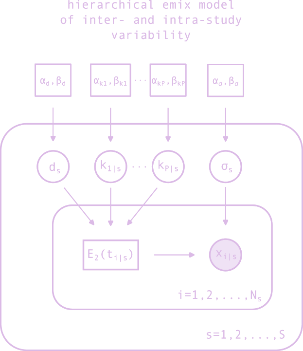
hierarchical emix model
data and inferences
twice-weekly patches
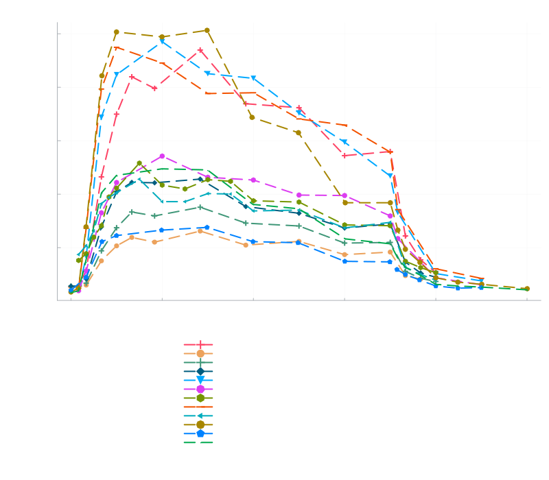
We collected and digitized the data from the following sources
- Houssain et al. 2003 - Dose proportionality study of four doses of an estradiol transdermal system, Estradot®
- Houssain et al. 2003 - Comparative bioequivalence studies with Estradot® and Menorest® transdermal systems
- Mylan Pharmaceuticals Inc. Mylan Estradiol patch drug label (updated January 12, 2022)
We perform the inference using the 3-compartments PK model and a normal data likelihood and individual random weights for each individual combination of (study, dose). We do not remove the baseline levels from the data and instead leave it as a parameter to be infered by the model. Once again each combination of (study, dose) gets their own random baseline level. We ignore the two data points at \(t=0\) in Houssain et al. 2003 with n=30 given the apparent decrease in serum level between hour 0 and hour 2. This dataset uses twice-weekly patches and we therefore set \(W = 3.5\).
appendix
general solution of the 3-compartments model
Consider the 3-compartment model again but this time with arbitrary pulses in all three compartments. One can think of this as modeling the effect of combining IM and IV injections of an estradiol ester together with IV injections of estradiol. This is not a recommended regimen and is used here purely for the sake of mathematical generality. We therefore write \begin{equation}\label{eq:general3Cdiffeq}\begin{split} \frac{dD(t)}{dt} &= -k_1 D(t) + \sum_i d_i \delta(t - t_i),\\ \frac{dE_s(t)}{dt} &= k_1 D(t) - k_2 E_s(t) + \sum_j d_j^s \delta(t - t_j),\\ \frac{dE_2(t)}{dt} & = k_2 E_s(t) - k_3 E_2(t) + \sum_k d^2_k\delta(t - t_k), \\ D(0) &= E_s(0) = E_2(0) = 0, \end{split}\end{equation} Here we assumed without loss of generality that the smallest among all \(t_i\)'s, \(t_j\)'s, and \(t_k\)'s is \(0^+\). It is easy to solve this system of ODEs using the Laplace transform since all processes are unidirectional and therefore we can proceed through simple forward substitution. Using the initial conditions \(D(0) = E_s(0) = E_2(0) = 0\) we can write the Laplace transform of the system of equations \begin{equation}\label{eq:general3Claplace}\begin{split} sD(s) &= -k_1 D(s) + \sum_i d_i e^{-s t_i},\\ sE_s(s) &= k_1 D(s) - k_2 E_s(s) + \sum_j d_j^s e^{-s t_j},\\ sE_2(s) & = k_2 E_s(s) - k_3 E_2(s) + \sum_k d^2_k e^{-s t_k}, \end{split}\end{equation} where by an abuse of notation we use \(D(s)\), \(E_s(s)\), and \(E_2(s)\) to denote the Laplace transforms of \(D(t)\), \(E_s(t)\), and \(E_2(t)\), respectively. We isolate \(D(s)\) in the first equation, \begin{equation}\label{eq:laplacefirstcompartment} D(s) = \frac{\sum_i d_i e^{-s t_i}}{s + k_1}, \end{equation} and notice that this is nothing but the Laplace transform of the convolution of a causal exponential and a shifted Dirac delta. We can therefore write the solution for the first compartmentSubstituting \eqref{eq:laplacefirstcompartment} in the second line of \eqref{eq:general3Claplace} we get \begin{equation} E_s(s) = \frac{k_1\sum_i d_i e^{-s t_i}}{(s + k_1)(s + k_2)} + \frac{\sum_j d_j^s e^{-s t_j}}{s + k_2}. \end{equation} Using partial fractions we decompose \begin{equation*} \frac{1}{(s + k_1)(s + k_2)} = -\frac{1}{(k_1 - k_2)(s + k_1)} + \frac{1}{(k_1 - k_2)(s + k_2)},\\ \end{equation*} and therefore \begin{equation}\label{eq:laplacesecondcompartment} E_s(s) = \frac{k_1}{k_1 - k_2}\sum_i d_i e^{-s t_i}\left[-\frac{1}{s + k_1} + \frac{1}{s + k_2}\right] + \frac{\sum_j d_j^s e^{-s t_j}}{s + k_2}. \end{equation} We notice once again that all those terms are nothing but Laplace transforms of convolutions of causal exponentials with shifted Dirac deltas and thus
Finally we isolate \(E_2(s)\) in the third line of \eqref{eq:general3Cdiffeq} and substitute \eqref{eq:laplacesecondcompartment} to get \begin{equation}\begin{split} E_2(s) &= \frac{k_2}{s + k_3} E_s(s) + \frac{\sum_k d_k^2 e^{-s t_k}}{s + k_3}, \\ &= \frac{k_1 k_2}{k_1 - k_2}\sum_i d_i e^{-s t_i}\left[\frac{1}{(s+k_2)(s+k_3)} - \frac{1}{(s+k_1)(s+k_3)}\right]\\ & + \frac{k_2 \sum_j d_j^se^{-st_j}}{(s + k_2)(s+k_3)} \\ & + \sum_k d^2_k \frac{e^{-st_k}}{s + k_3}. \end{split}\end{equation} Using once again all the same two tricks we finally obtain the general solution for the 3rd compartment